Evaluating Trading Strategies with Random Portfolios

Active asset management has been under attack during the past several months.  Hedge funds have been shutting down left and right, labeled as overpriced and underperforming, and are losing capital to low cost passive mutual funds and ETFs.  Active mutual funds have been losing ground as well to their passive counterparts. Warren Buffet has even gone so far as to refer to hedge fund managers who have a good track record for consecutive years as lucky monkey prophets and wants you to dismiss them immediately.

Most quant practitioners who have had first hand experience assisting discretionary portfolio managers in strategy development have a sense of where Buffet is coming from.  After working day in and day out with a portfolio manager for an extended period of time, one inevitably will develop an understanding of what market factors he believes are important, how he balances risk/reward tradeoffs, and ultimately how he makes trading decisions.  Over a career, one may have the opportunity to work with dozens of portfolio managers and there are some that convince us that they have found genuine sources of alpha and have a real skill.

Unfortunately for every one of these portfolio managers, there are nine other guys.  The other guy, you know what I mean?  He is the trader that works 16 hours a day,  never misses face-time with his boss, has mastered domineering everyone around him, has a sense of self confidence in his trading abilities that puts President Trump to shame, dresses like he is ready to strut down the catwalk at a moment’s notice, basks in a traditional hierarchical corporate workplace structure, and revels in reminding you that his title is Global MD Head of the Business and International CEO Partner, which means you are more junior, and he has been doing this for 20+ years.   You know the type, and let’s face it … this guy makes bad look good.  But after working side by side with him for several excruciating weeks which turn into months, you cannot help but notice that something is not right. Despite all the flamboyance, this guy really has no idea what he is doing.  He might as well be rolling a pair of dice to decide what securities to buy and sell.

How can one distinguish such a trader from a legitimate alpha generator?  One of the most common ways we do this in practice is to measure his performance relative to a benchmark or to his peers.  However this often leads to an apples to oranges style of comparison.  One alternative it to understand how well he performs when compared with strategies that have the same constraints that he is required by risk to stay within, but have randomly constructed trading rules.  In other words,  if we gather a group of Warren Buffet’s monkeys together and ask them to play a game with the same rules as those that we give to the trader, how well does the trader perform when compared with these peers?

 

We give a demonstration on how to design a random portfolio based performance metric below in the context of a simplified example.  Python code to run the Monte Carlo simulations outlined in subsequent sections that also produces the below plots is available here on Github as well as stock data for the S&P100 index that we use to demonstrate these ideas.

An All-Star Stock Trader?

Suppose it is 1/1/2010 and that you run a hedge fund and have just hired a new all-star trader.  He claims his expertise is in long only large cap stock picking over a multi-year time horizon and that he does not believe in hedging or market neutral strategies. Given this information, you ask him to distribute all his capital today among 10 stocks of his choosing from the S&P 100.  He then will have to follow a buy/hold strategy for the next six years and your risk team will monitor the risk profile and performance of his book on a daily basis.

Then you wait, and after the first year, you find he returns 11%, after the third 14.5% annualized, and after six years he levels off at a 12% annualized return.  All the while the trader regularly reminds you that he is crushing your credit, FX, and swaps teams, is carrying your firm, and now needs you to double his AUM.  How can we evaluate the performance of this PM before deciding whether or not to ramp up his capital?

We could compare him to the performance of the broader S&P100 market that he selected the stocks in his portfolio from, but we would rather try something a little more customized.  With this in mind, we decide to see how he compares against buy/hold trading strategies constructed by randomly selecting stocks from the index constituents.

A Random Portfolio Monte Carlo Simulation

First, we select a random subset of 10 stocks from the index and generate a normalized vector of weights whose components are i.i.d. draws from a standard uniform distribution.  We then compute the simple returns of each stock and take a weighted sum to find the daily returns of the portfolio.  From this, we estimate the annualized return, volatility, and Sharpe ratio using a 252 day lookback window on a rolling basis and store the resulting Sharpe ratio time series.  Then we repeat this process 10,000 times. Finally, we compute the mean and standard deviation of the set of 10,000 points associated with each day in the six year holding period and plot the mean series in the below figure in blue and the 2 standard deviation series on both sides of the mean in grey.

The first thing that we note is that our random portfolios did quite well.  They had a respectable Sharpe Ratio above 1 for more than half the trading period and seldom had negative year-on-year returns.  However, we also note that the distance between the upper and lower grey error curves is quite small.  It ranges from being nearly zero to around 0.5 Sharpe ratio points and has an average value of approximately 0.2.  That is to say that 95% of all buy/hold trading strategies consisting of 10 stocks have a SR that is on average within 0.1 of the Sharpe ratio of the average strategy at any point in time.  This seems to make things quite difficult for the trader to distinguish himself as it seems all trading strategies appear to be closely related to one another.

Let us look into a few further descriptive statistics and performance measures of this trading strategies but now only considering the full six year time window and varying the number of securities that a trader is allowed to hold.  First, we take the last point of the cumulative return series of each random portfolio and annualize it.  We then plot the histogram (with the help of seaborn’s dist_plot function which overlays a kernel density estimate on top of the histogram) and then repeat the same experiment for portfolios of 2, 5, 20, 50, and 95 securities and plot the results in the figure below.

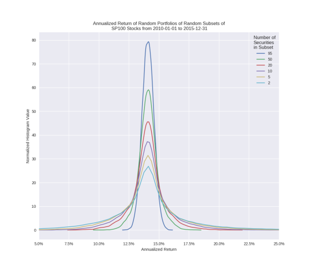
Notice how as we increase the number of securities, the variance of the expected annualized return distribution decreases.  This shows us that the more securities we have to hold in our portfolio, the more difficult it becomes to have very high (say 20%+) returns.  We also see that our all-star trader’s 12% return does not look as impressive as he claims.  In particular, he is approximately in the 20-30%-ile when compared with the results of our army of 10,000 monkeys.

Next, let’s look at how the annualized volatility of these strategies are distributed. Specifically, we compute the standard deviation of the returns of each random portfolio on a rolling window and then annualize by multiplying by a factor of and then repeat for varying numbers of securities and plot the results below.

Note that the distributions are skewed to the right.  It appears that it is quite difficult to achieve vols lower than 14%, most strategies have volatility in the 15-16.5% range, and there are a few strategies with a low number of securities that have high 22%+ vol.  Note how these distributions also localize as the number of stocks selected increases which gives a demonstration of the diversification benefits of a larger portfolio.

Dividing the annualized return by the volatility in each of the two above examples, we plot the distribution of Sharpe ratios for each simulation.

Note that the very few strategies have a vol lower than 14% which seems to prevent the vol from being small enough to allow for strategies with high 2+ Sharpe ratios.  Also, the right skew in the vol distributions creates a left half skew in the Sharpe Ratio distributions.  From this plot, we can see that is it quite difficult to construct a poorly performing strategy within our model constraints even if one set out to do so from the onset. Specifically, the majority of Sharpe ratios are within the respectable range of 0.8 to 1.0.

Finally, we compute the maximum peak-to-trough drawdown of each of our simulated strategies and plot the results below.

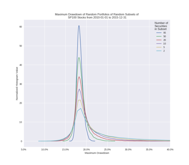
The results are not good as is seems typically max drawdowns are in the 15-20% range. Strategies tend to be shut down on the buyside once their max drawdowns start to exceed 5%, unless extenuating circumstances exist, which seems to spell the end for our long only strategy.

Limitations, Extensions, and Conclusions

The above is a simplified example that would not be reasonable to implement in practice.  Specifically the vast majority of equity strategies being run at hedge funds are long/short market neutral with strict beta limits designed to prohibit portfolio managers from taking directional bets on the market or individual sectors.  In addition, active trading on varying frequencies is more realistic than a buy/hold strategies. However, given the set of securities a portfolio manager trades in, risk constraints on his strategy, and a  rough model of his trading behavior, one can construct a related Monte Carlo simulation of random portfolios which tries to capture the trading style as close as possible and also accounts for additional features such as transaction costs and market impact.  This allows for the construction of one additional performance metric on which to evaluate the performance of the strategy.